From Raw Roads to Intelligent Routing with PostGIS & pgRouting
An end-to-end SQL-based routing pipeline using PostgreSQL, PostGIS, and pgRouting — transforming raw road geometries into a production-ready network for shortest path analysis.
From Raw Roads to Intelligent Routing: Building a pipeline with PgRouting and PostGIS
🛠️ Code Resources and Full SQL Pipeline
All SQL steps and source code used in this project are accessible via the links below:
| Description | Link |
|---|---|
| Full Sample Project Repository | GitHub Project Repository (shortest-route-mvp) |
| Step-by-Step SQL Pipeline (Markdown) | postgresql_postgis_pgrouting_shortest_path_pipeline.md |
As a GIS & software engineer, one of the most common yet underestimated problems I see in projects is routing.
“We already have road data, how hard can shortest path be?”
In practice, routing is not about having lines on a map — it’s about turning geometry into a mathematically correct, performant graph.
In this post, I’ll walk through an end‑to‑end PostgreSQL + PostGIS + pgRouting pipeline that transforms raw road geometries into a fully routable network and computes shortest paths using both Dijkstra and A*.
This approach is pure SQL, production‑ready, and works perfectly behind WebGIS stacks such as GeoServer, REST APIs, or custom frontend frameworks.
Why This Pipeline Matters
Many routing examples skip critical steps:
- Missing intersection handling
- Incorrect node creation
- Invalid graph topology
- Poor performance at scale
This workflow explicitly solves those problems by:
- Creating true network nodes (vertices + intersections)
- Splitting roads into atomic routable edges
- Supporting dynamic user‑defined start/end points
1. Verifying the Spatial Stack
Before touching data, always confirm your environment:
- PostgreSQL
- PostGIS
- pgRouting
A quick query against pg_extension ensures everything is installed and versioned correctly.
This step sounds trivial, but it prevents painful debugging later — especially in containerized or enterprise environments.
2. Roads Are Geometry, Not a Network
We start with a simple road table storing LINESTRING geometries in WGS84.
At this stage:
- Roads may overlap
- Lines may cross without nodes
- Endpoints may not align
From a routing perspective, this is not a graph yet.
3. Turning Lines into Nodes
A routable network needs nodes.
We generate nodes from two sources:
a) Line vertices
Every vertex along a road can potentially be a decision point.
Using ST_DumpPoints, we extract all vertices and store them as points.
b) Road intersections
Intersections are critical.
Even if two roads cross visually, routing will fail unless there is a shared node.
By intersecting every road with every other road and filtering for point geometries, we create explicit intersection nodes.
4. Cleaning and Indexing Nodes
Raw node extraction creates duplicates.
We normalize the node table by:
- Removing duplicates
- Enforcing uniqueness
- Adding spatial indexes
This dramatically improves nearest‑node searches later — especially for dynamic routing.
5. Building Network Edges (The Core Step)
This is where most routing pipelines fail.
The challenge
Each road must be split into ordered segments between nodes.
The solution
- Project nodes onto each road
- Compute their relative position using
ST_LineLocatePoint - Sort nodes along the line
- Connect consecutive node pairs
Each segment becomes an edge with:
sourcenodetargetnode- geometry
- cost
This guarantees a topologically correct graph.
6. Cost Calculation: Real Distance
Costs are computed using:
ST_DistanceSphere- Converted to kilometers
- Rounded for stability
This gives realistic routing results without projection headaches.
7. Reverse Cost: The pgRouting Rule
pgRouting always expects:
costreverse_cost
Even if your network is undirected.
By assigning equal forward and reverse costs, we model bi‑directional roads correctly.
Skipping this step is one of the most common pgRouting mistakes.
8. Static Shortest Path (Node IDs)
Once the graph is ready, classic Dijkstra works immediately.
Given two node IDs, pgRouting returns the ordered list of edges forming the shortest path.
At this point, your database is officially a routing engine.
9. Dynamic Routing with User Points
Real applications don’t know node IDs.
They know:
- A clicked point
- A GPS coordinate
- A request payload
The approach
- Store user points
- Find nearest network nodes using KNN (
<->) - Run routing between those nodes
All handled inside SQL.
10. Materialized Views for Performance
Routing queries can be expensive.
Materialized views allow:
- Pre‑computed routes
- Fast map rendering
- Controlled refresh cycles
This pattern works extremely well with:
- GeoServer WMS/WFS
- Vector tiles
- Backend APIs
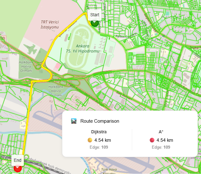
Dijkstra vs A*
Both are implemented in this pipeline:
- Dijkstra: guaranteed optimal, slower on large graphs
- A*: faster using heuristics, ideal for interactive apps
Because the graph is clean, switching algorithms is trivial.
Where This Fits in Real Systems
I’ve successfully used this exact pattern in:
- WebGIS routing services
- Fleet & logistics systems
- Urban analysis platforms
- Military & enterprise GIS environments
It scales, it’s transparent, and it keeps routing logic where it belongs: in the database.
Final Thoughts
Routing is not magic.
It’s careful topology, solid geometry handling, and disciplined SQL.
If you treat road data as just lines, routing will betray you. If you treat it as a graph — it becomes one of the most powerful tools in spatial engineering.
If you want, next we can:
- Expose this via a REST API
- Serve it through GeoServer
- Visualize it in Angular + Cesium
- Optimize it for millions of edges
Happy routing 🚀
Prepared by Burhan Sözer
GIS & Software Engineer